
GET TO KNOW THE STEPS OF THE MAPBIOMAS METHODOLOGY
Here we detail the MapBiomas Atlantic Forest methodology step by step. For each class treated in the map there are specific peculiarities and characteristics that can be checked in detail in the ATBD in its appendices.
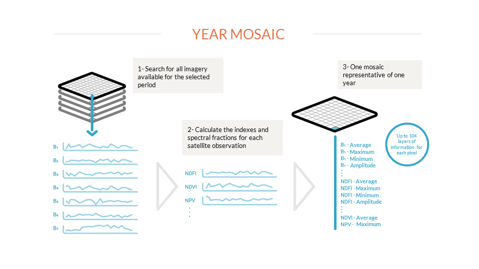
It all starts with Landsat satellite imagery, with 30-meter resolution, available for free on the Google Earth Engine platform and with a time series of more than 30 years. Images can contain clouds, smoke, and other artifacts that can “dirty” them. To produce a clean image, the cloudless pixels are selected from the available images for the selected period. For each of these pixels are extracted metrics that explain the behavior of the pixel in that year. This is done with each of the 7 satellite spectral bands as well as for the calculated spectral fractions and indices. For example, for Band 1 the median of band values in the period, the maximum value, the minimum value in the year and the amplitude of variation is collected. At the end each pixel for one year carries up to 104 layers of information.
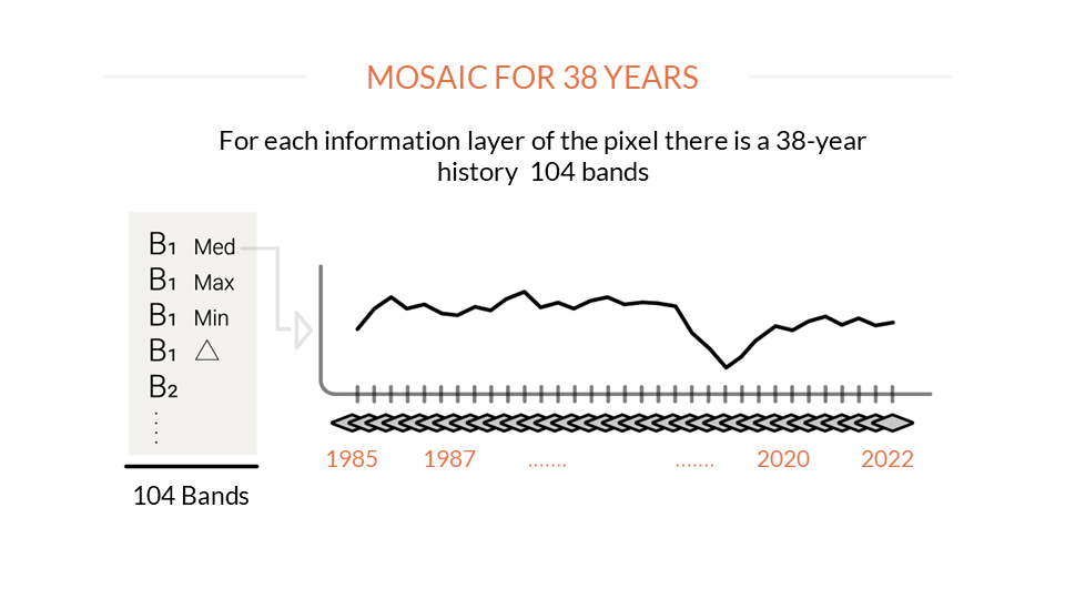
For each year a mosaic covering Atlantic Forest biome is set up representing the behavior of each pixel through 104 metrics or layers of information. This mosaic set is saved as a collection of data (Asset) within the Google Earth Engine platform. These mosaics will be used in two main ways. First as source parameters for the algorithm to produce classification (see next step). It is also from this mosaic that RGB composition is derived allowing to visualization of the background image in the platform MapBiomas. This composition is also used for the collection of training samples and samples for assessment of accuracy by visual interpretation.
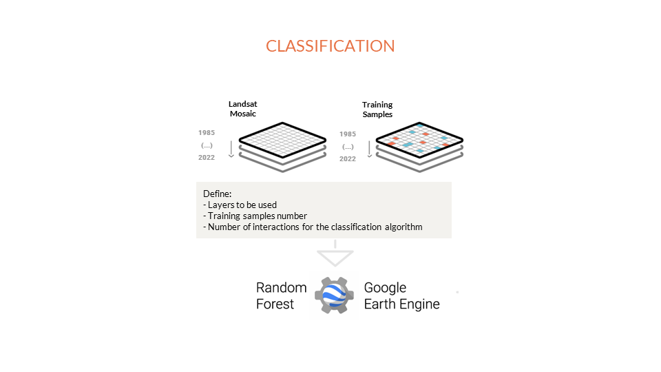
From the image mosaics, the land cover and use map (forest, field, agriculture, pasture, urban area, water, etc.) is made. To do so, MapBiomas analysts use an automatic classifier called “random forest”, which runs on Google Earth Engine. This system is based on machine learning: for each topic to be classified, the machines are “trained” with samples of the targets to be classified. These samples are obtained by means of reference maps, generation of maps of stable classes of the previous series of MapBiomas Atlantic Forest and by direct collection by visual interpretation of the Landsat images.
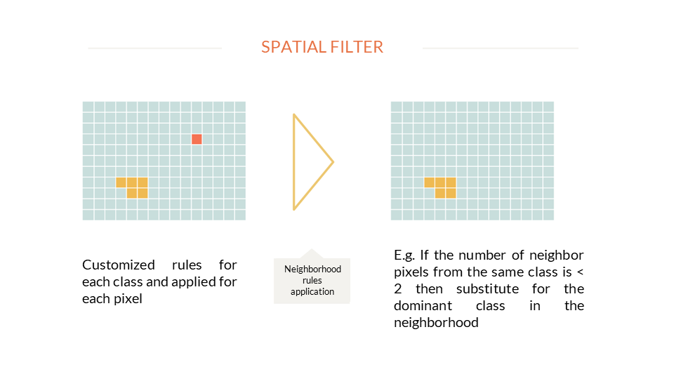
The spatial filter aims to increase the spatial consistency of the data by eliminating isolated or border pixels. Neighborhood rules are defined that can lead to a change in pixel classification. For example, a pixel that has less than two out of the nine neighboring pixels in the same class will be reclassified to the predominant class in the neighborhood. The filter applies to all classes and years in the collection
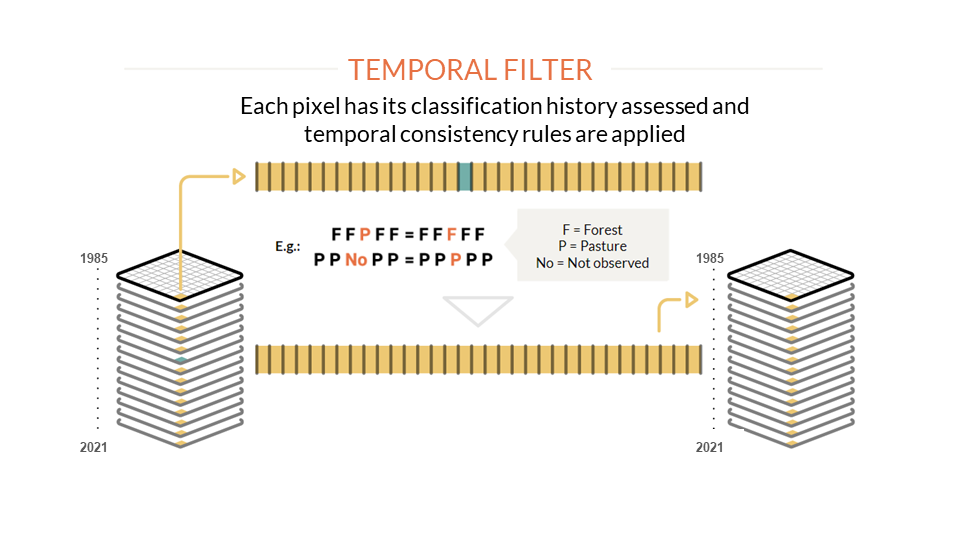
In order to reduce temporal inconsistencies, in particular changes in coverage and use that are impossible or not permitted (eg Natural Forest > Non-Forest > Natural Forest) and to correct failures due to cloud overflow or lack of data, a temporal filter is applied. Each biome, theme or region may have specific temporal filter rules. The temporal filter is applied to each pixel analyzing all the years of the Collection (eg Collection 3 are 38 years).
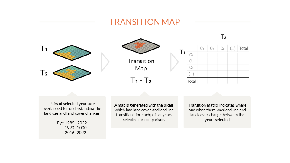
In order to understand changes in land cover and land use, maps are produced with class transitions between different pairs of selected years. It is thus possible to visualize the dynamism of the territory, and answer questions such as how much of the forest has turned pasture from one year to another, for example, among other changes in the landscape. Transition maps are produced pixel by pixel and after finalized also pass through a spatial filter to eliminate isolated transition or border pixels. From these maps are constructed the transition matrices for each administrative unit, available on the MapBiomas Atlantic Forest platform.